Student's t-distribution

Student's t

Probability density function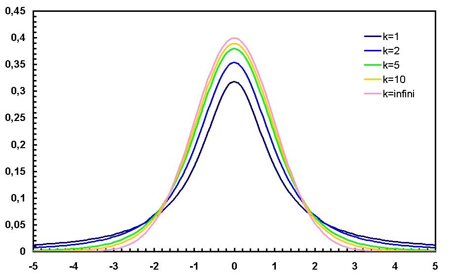
Cumulative distribution function
Parameters	$\nu > 0\!$ deg. of freedom (real)
Support	$x \in (-\infty;+\infty)\!$
pdf	$\frac{\Gamma((\nu+1)/2)} {\sqrt{\nu\pi}\,\Gamma(\nu/2)\,(1+x^2/\nu)^{(\nu+1)/2}}\!$
cdf	$\frac{1}{2} + \frac{x \Gamma \left( (\nu+1)/2 \right) 2\, F_1 \left ( \frac{1}{2},(\nu+1)/2;\frac{3}{2};-\frac{x^2}{\nu} \right)} {\sqrt{\pi\nu}\,\Gamma (\nu/2)}$
Mean	$0$
Median	$0$
Mode	$0$
Variance	$\frac{\nu}{\nu-2}\!$ for $\nu>2$
Skewness	$0$ for $\nu>3$
Kurtosis	$\frac{6}{\nu-4}\!$ for $\nu>4$
Entropy	$\begin{matrix} \frac{\nu+1}{2}\left[ \psi(\frac{1+\nu}{2}) - \psi(\frac{\nu}{2}) \right] \\[0.5em] + \log{\left[\sqrt{\nu}B(\frac{\nu}{2},\frac{1}{2})\right]} \end{matrix}$ $\psi$: digamma function, $B$: beta function
mgf	see text for raw/central moments
Char. func.

In probability and statistics, the t-distribution or Student's t-distribution is a probability distribution that arises in the problem of estimating the mean of a normally distributed population when the sample size is small. It is the basis of the popular Student's t-tests for the statistical significance of the difference between two sample means, and for confidence intervals for the difference between two population means. The Student's t-distribution is a special case of the generalised hyperbolic distribution.

Although the t-distribution is attributed to William Sealy Gosset, it was actually first derived as a posterior distribution in 1876 by Helmert and Luroth. Before William Gosset published the derivation of t-distribution, it also appeared in a more general form as Pearson Type IV in Karl Pearson's 1895 paper. In English literature, the derivation of the t-distribution was first published in 1908 by William Sealy Gosset, while he worked at a Guinness brewery in Dublin. He published it in the paper Biometrika and as he was not allowed to publish under his own name, he penned it under the pseudonym Student. The t-test and the associated theory became well-known through the work of R.A. Fisher, who called the distribution "Student's distribution".

Student's distribution arises when (as in nearly all practical statistical work) the population standard deviation is unknown and has to be estimated from the data. Textbook problems treating the standard deviation as if it were known are of two kinds: (1) those in which the sample size is so large that one may treat a data-based estimate of the variance as if it were certain, and (2) those that illustrate mathematical reasoning, in which the problem of estimating the standard deviation is temporarily ignored because that is not the point that the author or instructor is then explaining.

Occurrence and specification of Student's t-distribution

Suppose X₁, ..., X_n are independent random variables that are normally distributed with expected value μ and variance σ². Let

$\overline{X}_n=(X_1+\cdots+X_n)/n$

be the sample mean, and

${S_n}^2=\frac{1}{n-1}\sum_{i=1}^n\left(X_i-\overline{X}_n\right)^2$

be the sample variance. It is readily shown that the quantity

$Z=\frac{\overline{X}_n-\mu}{\sigma/\sqrt{n}}$

is normally distributed with mean 0 and variance 1. Gosset studied a related quantity,

$T=\frac{\overline{X}_n-\mu}{S_n/\sqrt{n}}$

and showed that T has the probability density function

$f(t) = \frac{\Gamma((\nu+1)/2)}{\sqrt{\nu\pi\,}\,\Gamma(\nu/2)} (1+t^2/\nu)^{-(\nu+1)/2}$

with

$\nu$ equal to n − 1. The distribution of T is now called the t-distribution.

The parameter

$\nu$ is conventionally called the number of degrees of freedom. The distribution depends on

$\nu$ , but not

$\mu$ or

$\sigma$

the lack of dependence on

$\mu$ and

$\sigma$ is what makes the t-distribution important in both theory and practice.

$\Gamma$ is the Gamma function.

Confidence intervals derived from Student's t-distribution

Suppose the number A is so chosen that

$\Pr(-A < T < A)=0.9,\,$

when T has a t-distribution with n − 1 degrees of freedom (this is the same as

$\Pr(T < A) = 0.95,\,$

so A is the "95th percentage point" of this probability distribution). Then

$\Pr\left(-A < {\overline{X}_n - \mu \over S_n/\sqrt{n}} < A\right)=0.9,$

and this is equivalent to

$\Pr\left(\overline{X}_n - A{S_n \over \sqrt{n}} < \mu < \overline{X}_n + A{S_n \over \sqrt{n}}\right) = 0.9.$

Therefore the interval whose endpoints are

$\overline{X}_n\pm A\frac{S_n}{\sqrt{n}}$

is a 90-percent confidence interval for μ. Therefore, if we find the mean of a set of observations that we can reasonably expect to have a normal distribution, we can use the t-distribution to examine whether the confidence limits on that mean include some theoretically predicted value - such as the value predicted on a null hypothesis.

It is this result that is used in the Student's t-tests: since the difference between the means of samples from two normal distributions is itself distributed normally, the t-distribution can be used to examine whether that difference can reasonably be supposed to be zero.

If the data is normally distributed, the one-sided (1 − a)-upper confidence limit (UCL) of the mean, can be calculated using the following equation:

$\mathrm{UCL}_{1-a} = \overline{X}_n+\frac{t_{a,n-1} S}{\sqrt{n}}.$

The resulting UCL will be the greatest average value that will occur for a given confidence interval and population size. In other words,

$\overline{X}_n$ being the mean of the set of observations, the probability that the mean of the distribution is inferior to

$\mathrm{UCL}_{1-a}$ is equal to the confidence level

$1-a.$

A number of other statistics can be shown to have t-distributions for samples of moderate size under null hypotheses that are of interest, so that the t-distribution forms the basis for significance tests in other situations as well as when examining the differences between means. For example, the distribution of Spearman's rank correlation coefficient, rho, in the null case (zero correlation) is well approximated by the t distribution for sample sizes above about 20.

See prediction interval for another example of the use of this distribution.

Further theory

Gosset's result can be stated more generally. (See, for example, Hogg and Craig, Sections 4.4 and 4.8.) Let Z have a normal distribution with mean 0 and variance 1. Let V have a chi-square distribution with ν degrees of freedom. Further suppose that Z and V are independent (see Cochran's theorem). Then the ratio

$\frac{Z}{\sqrt{V/\nu\ }}$

has a t-distribution with ν degrees of freedom.

For a t-distribution with ν degrees of freedom, the expected value is 0, and its variance is ν/(ν − 2) if ν > 2. The skewness is 0 and the kurtosis is 6/(ν − 4) if ν > 4.

The cumulative distribution function is given by an incomplete beta function,

$\int_{-\infty}^t f(u)\,du = \left\{ \begin{matrix} 1 - \frac{1}{2} I_x(\nu/2,1/2) & \mbox{if}\quad t > 0, \\ \\ \frac{1}{2} I_x(\nu/2,1/2) & \mbox{otherwise}, \end{matrix}\right.$

with

$x = \frac{1}{1+t^2/\nu}.$

The t-distribution is related to the F-distribution as follows: the square of a value of t with ν degrees of freedom is distributed as F with 1 and ν degrees of freedom.

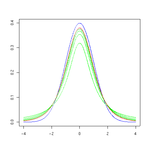
The overall shape of the probability density function of the t-distribution resembles the bell shape of a normally distributed variable with mean 0 and variance 1, except that it is a bit lower and wider. As the number of degrees of freedom grows, the t-distribution approaches the normal distribution with mean 0 and variance 1.

The following images show the density of the t-distribution for increasing values of ν. The normal distribution is shown as a blue line for comparison.; Note that the t-distribution (red line) becomes closer to the normal distribution as ν increases. For ν = 30 the t-distribution is almost the same as the normal distribution.

Density of the t-distribution (red and green) for 1, 2, 3, 5, 10, and 30 df compared to normal distribution (blue)

Table of selected values

The following table lists a few selected values for distributions with r degrees of freedom for the 90%, 95%, 97.5%, and 99.5% confidence intervals. These are "one-sided", i.e., where we see "90%", "4 degrees of freedom", and "1.533",

it means Pr(T < 1.533) = 0.9;

it does not mean Pr(−1.533 < T < 1.533) = 0.9.

Consequently, by the symmetry of this distribution, we have

Pr(−1.533 < T) = 0.9,

and consequently

Pr(−1.533 < T < 1.533) = 0.8.

r	75%	80%	85%	90%	95%	97.5%	99%	99.5%	99.75%	99.9%	99.95%
1	1.000	1.376	1.963	3.078	6.314	12.71	31.82	63.66	127.3	318.3	636.6
2	0.816	1.061	1.386	1.886	2.920	4.303	6.965	9.925	14.09	22.33	31.60
3	0.765	0.978	1.250	1.638	2.353	3.182	4.541	5.841	7.453	10.21	12.92
4	0.741	0.941	1.190	1.533	2.132	2.776	3.747	4.604	5.598	7.173	8.610
5	0.727	0.920	1.156	1.476	2.015	2.571	3.365	4.032	4.773	5.893	6.869
6	0.718	0.906	1.134	1.440	1.943	2.447	3.143	3.707	4.317	5.208	5.959
7	0.711	0.896	1.119	1.415	1.895	2.365	2.998	3.499	4.029	4.785	5.408
8	0.706	0.889	1.108	1.397	1.860	2.306	2.896	3.355	3.833	4.501	5.041
9	0.703	0.883	1.100	1.383	1.833	2.262	2.821	3.250	3.690	4.297	4.781
10	0.700	0.879	1.093	1.37218	1.812	2.228	2.764	3.169	3.581	4.144	4.587
11	0.697	0.876	1.088	1.363	1.796	2.201	2.718	3.106	3.497	4.025	4.437
12	0.695	0.873	1.083	1.356	1.782	2.179	2.681	3.055	3.428	3.930	4.318
13	0.694	0.870	1.079	1.350	1.771	2.160	2.650	3.012	3.372	3.852	4.221
14	0.692	0.868	1.076	1.345	1.761	2.145	2.624	2.977	3.326	3.787	4.140
15	0.691	0.866	1.074	1.341	1.753	2.131	2.602	2.947	3.286	3.733	4.073
16	0.690	0.865	1.071	1.337	1.746	2.120	2.583	2.921	3.252	3.686	4.015
17	0.689	0.863	1.069	1.333	1.740	2.110	2.567	2.898	3.222	3.646	3.965
18	0.688	0.862	1.067	1.330	1.734	2.101	2.552	2.878	3.197	3.610	3.922
19	0.688	0.861	1.066	1.328	1.729	2.093	2.539	2.861	3.174	3.579	3.883
20	0.687	0.860	1.064	1.325	1.725	2.086	2.528	2.845	3.153	3.552	3.850
21	0.686	0.859	1.063	1.323	1.721	2.080	2.518	2.831	3.135	3.527	3.819
22	0.686	0.858	1.061	1.321	1.717	2.074	2.508	2.819	3.119	3.505	3.792
23	0.685	0.858	1.060	1.319	1.714	2.069	2.500	2.807	3.104	3.485	3.767
24	0.685	0.857	1.059	1.318	1.711	2.064	2.492	2.797	3.091	3.467	3.745
25	0.684	0.856	1.058	1.316	1.708	2.060	2.485	2.787	3.078	3.450	3.725
26	0.684	0.856	1.058	1.315	1.706	2.056	2.479	2.779	3.067	3.435	3.707
27	0.684	0.855	1.057	1.314	1.703	2.052	2.473	2.771	3.057	3.421	3.690
28	0.683	0.855	1.056	1.313	1.701	2.048	2.467	2.763	3.047	3.408	3.674
29	0.683	0.854	1.055	1.311	1.699	2.045	2.462	2.756	3.038	3.396	3.659
30	0.683	0.854	1.055	1.310	1.697	2.042	2.457	2.750	3.030	3.385	3.646
40'	0.681	0.851	1.050	1.303	1.684	2.021	2.423	2.704	2.971	3.307	3.551
50	0.679	0.849	1.047	1.299	1.676	2.009	2.403	2.678	2.937	3.261	3.496
60	0.679	0.848	1.045	1.296	1.671	2.000	2.390	2.660	2.915	3.232	3.460
80	0.678	0.846	1.043	1.292	1.664	1.990	2.374	2.639	2.887	3.195	3.416
100	0.677	0.845	1.042	1.290	1.660	1.984	2.364	2.626	2.871	3.174	3.390
120	0.677	0.845	1.041	1.289	1.658	1.980	2.358	2.617	2.860	3.160	3.373
$\infty$	0.674	0.842	1.036	1.282	1.645	1.960	2.326	2.576	2.807	3.090	3.291

For example, given a sample with a sample variance 2 and sample mean of 10, taken from a sample set of 11 (10 degrees of freedom), using the formula:

$\overline{X}_n\pm A\frac{S_n}{\sqrt{n}}$

We can determine that at 90% confidence, we have a true mean lying below:

$10+1.37218 \frac{\sqrt{2}}{\sqrt{11}}=10.58510$

And, still at 90% confidence, we have a true mean lying over:

$10-1.37218 \frac{\sqrt{2}}{\sqrt{11}}=9.41490$

So that at 80% confidence, we have a true mean lying between

$10\pm1.37218 \frac{\sqrt{2}}{\sqrt{11}}=[9.41490,10.58510]$

Special cases

Certain values of

$\nu$ give an especially simple form.

$\nu=1$Distribution function

$F(x) = \frac{1}{2} + \frac{1}{\pi}\tan^{-1}(x)$

$\nu=2$Distribution function

$F(x) = \frac{1}{2}\left[1+\frac{x}{\sqrt{2+x^2}}\right]$

Density function

$f(x) = \frac{1}{\left(2+x^2\right)^{3/2}}$

Related distributions

• $Y \sim \mathrm{F}(\nu_1 = 1, \nu_2 = \nu)$is a F-distribution if$Y = X^2 \,$ and$X \sim \mathrm{t}(\nu)$ is a Student's t-distribution.
• $Y \sim N(0,1)$is a normal distribution as$Y = \lim_{\nu \to \infty} X$ where$X \sim \mathrm{t}(\nu)$.
• $X \sim \mathrm{Cauchy}(0,1)$is a Cauchy distribution if$X \sim \mathrm{t}(\nu = 1)$.

See also

• Gamma function
• Hotelling's T-square distribution
• Noncentral t-distribution

References

• "Student" (W.S. Gosset) (1908) The probable error of a mean. Biometrika 6(1):1--25.
• M. Abramowitz and I. A. Stegun, eds. (1972) Handbook of Mathematical Functions with Formulas, Graphs, and Mathematical Tables. New York: Dover. (See Section 26.7.)
• R.V. Hogg and A.T. Craig (1978) Introduction to Mathematical Statistics. New York: Macmillan.
•  Helmert FR (1875). "Über die Berechnung des wahrscheinlichen Fehlers aus einer endlichen Anzahl wahrer Beobachtungsfehler". Z. Math. U. Physik. 20: 300–3.
• Lüroth J (1876). "Vergleichung von zwei Werten des wahrscheinlichen Fehlers". Astron. Nachr. 87 (14): 209–20. Bibcode:1876AN.....87..209L. doi:10.1002/asna.18760871402.
• T Table | History of T Table, Etymology, one-tail T Table, two-tail T Table and T-statistic
• Pearson, K. (1895-01-01). "Contributions to the Mathematical Theory of Evolution. II. Skew Variation in Homogeneous Material". Philosophical Transactions of the Royal Society A: Mathematical, Physical and Engineering Sciences. 186: 343–414 (374). doi:10.1098/rsta.1895.0010. ISSN 1364-503X.
• Wendl MC (2016). "Pseudonymous fame". Science. 351 (6280): 1406. doi:10.1126/science.351.6280.1406. PMID 27013722.

External links

• VassarStats Density plot, critical values, etc., calculated for a user-specified number of d.f.
• Earliest Known Uses of Some of the Words of Mathematics (S) (Remarks on the history of the term "Student's distribution")
• Distribution Calculator Calculates probabilities and critical values for normal, t-, chi2- and F-distribution

de:Students t-Verteilung su:Sebaran-t student nl:Student-verdeling fr: Loi de Student