No edit summary |
(Take out machine learning) |
||
| Line 2: | Line 2: | ||
'''Data clustering''' is a common technique for [[statistics|statistical]] [[data analysis]], which is used in many fields, including [[machine learning]], [[data mining]], [[pattern recognition]], [[image analysis]] and [[bioinformatics]]. Clustering is the [[classification]] of similar objects into different groups, or more precisely, the [[partition of a set|partitioning]] of a data set into [[subset]]s (clusters), so that the data in each subset (ideally) share some common trait - often proximity according to some defined [[metric (mathematics)|distance measure]]. |
'''Data clustering''' is a common technique for [[statistics|statistical]] [[data analysis]], which is used in many fields, including [[machine learning]], [[data mining]], [[pattern recognition]], [[image analysis]] and [[bioinformatics]]. Clustering is the [[classification]] of similar objects into different groups, or more precisely, the [[partition of a set|partitioning]] of a data set into [[subset]]s (clusters), so that the data in each subset (ideally) share some common trait - often proximity according to some defined [[metric (mathematics)|distance measure]]. |
||
| + | |||
| − | Machine learning typically regards data clustering as a form of [[unsupervised learning]]. |
||
Besides the term ''data clustering'' (or just ''clustering''), there are a number of terms with similar meanings, including ''cluster analysis'', ''automatic classification'', ''numerical taxonomy'', ''botryology'' and ''typological analysis''. |
Besides the term ''data clustering'' (or just ''clustering''), there are a number of terms with similar meanings, including ''cluster analysis'', ''automatic classification'', ''numerical taxonomy'', ''botryology'' and ''typological analysis''. |
||
Revision as of 13:55, 30 July 2006
Assessment |
Biopsychology |
Comparative |
Cognitive |
Developmental |
Language |
Individual differences |
Personality |
Philosophy |
Social |
Methods |
Statistics |
Clinical |
Educational |
Industrial |
Professional items |
World psychology |
Statistics: Scientific method · Research methods · Experimental design · Undergraduate statistics courses · Statistical tests · Game theory · Decision theory
Data clustering is a common technique for statistical data analysis, which is used in many fields, including machine learning, data mining, pattern recognition, image analysis and bioinformatics. Clustering is the classification of similar objects into different groups, or more precisely, the partitioning of a data set into subsets (clusters), so that the data in each subset (ideally) share some common trait - often proximity according to some defined distance measure.
Besides the term data clustering (or just clustering), there are a number of terms with similar meanings, including cluster analysis, automatic classification, numerical taxonomy, botryology and typological analysis.
Types of clustering
Data clustering algorithms can be hierarchical or partitional. Hierarchical algorithms find successive clusters using previously established clusters, whereas partitional algorithms determine all clusters at once. Hierarchical algorithms can be agglomerative (bottom-up) or divisive (top-down). Agglomerative algorithms begin with each element as a separate cluster and merge them in successively larger clusters. Divisive algorithms begin with the whole set and proceed to divide it into successively smaller clusters.
Hierarchical clustering
Distance measure
A key step in a hierarchical clustering is to select a distance measure. A simple measure is manhattan distance, equal to the sum of absolute distances for each variable. The name comes from the fact that in a two-variable case, the variables can be plotted on a grid that can be compared to city streets, and the distance between two points is the number of blocks a person would walk.
A more common measure is Euclidean distance, computed by finding the square of the distance between each variable, summing the squares, and finding the square root of that sum. In the two-variable case, the distance is analogous to finding the length of the hypotenuse in a triangle; that is, it is the distance "as the crow flies." A review of cluster analysis in health psychology research found that the most common distance measure in published studies in that research area is the Euclidean distance or the squared Euclidean distance.
Creating clusters
Given a distance measure, elements can be combined. Hierarchical clustering builds (agglomerative), or breaks up (divisive), a hierarchy of clusters. The traditional representation of this hierarchy is a tree data structure (called a dendrogram), with individual elements at one end and a single cluster with every element at the other. Agglomerative algorithms begin at the top of the tree, whereas divisive algorithms begin at the bottom. (In the figure, the arrows indicate an agglomerative clustering.)
Cutting the tree at a given height will give a clustering at a selected precision. In the following example, cutting after the second row will yield clusters {a} {b c} {d e} {f}. Cutting after the third row will yield clusters {a} {b c} {d e f}, which is a coarser clustering, with a fewer number of larger clusters.
Agglomerative hierarchical clustering
For example, suppose this data is to be clustered. Where euclidean distance is the distance metric.
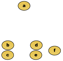
Raw data
The hierarchical clustering dendrogram would be as such:
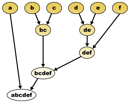
Traditional representation
This method builds the hierarchy from the individual elements by progressively merging clusters. Again, we have six elements {a} {b} {c} {d} {e} and {f}. The first step is to determine which elements to merge in a cluster. Usually, we want to take the two closest elements, therefore we must define a distance between elements. One can also construct a distance matrix at this stage.

Suppose we have merged the two closest elements b and c, we now have the following clusters {a}, {b, c}, {d}, {e} and {f}, and want to merge them further. But to do that, we need to take the distance between {a} and {b c}, and therefore define the distance between two clusters. Usually the distance between two clusters and is one of the following:


- The maximum distance between elements of each cluster (also called complete linkage clustering):

- The minimum distance between elements of each cluster (also called single linkage clustering):

- The mean distance between elements of each cluster (also called average linkage clustering):

- The sum of all intra-cluster variance
- The increase in variance for the cluster being merged (Ward's criterion)
- The probability that candidate clusters spawn from the same distribution function (V-linkage)
Each agglomeration occurs at a greater distance between clusters than the previous agglomeration, and one can decide to stop clustering either when the clusters are too far apart to be merged (distance criterion) or when there is a sufficiently small number of clusters (number criterion).
Partitional clustering
k-means and derivatives
K-means clustering
The K-means algorithm assigns each point to the cluster whose center (also called centroid) is nearest. The center is the average of all the points in the cluster — that is, its coordinates are the arithmetic mean for each dimension separately over all the points in the cluster.
- Example: The data set has three dimensions and the cluster has two points: X = (x1, x2, x3) and Y = (y1, y2, y3). Then the centroid Z becomes Z = (z1, z2, z3), where z1 = (x1 + y1)/2 and z2 = (x2 + y2)/2 and z3 = (x3 + y3)/2.
The algorithm is roughly (J. MacQueen, 1967):
- Randomly generate k clusters and determine the cluster centers, or directly generate k seed points as cluster centers.
- Assign each point to the nearest cluster center.
- Recompute the new cluster centers.
- Repeat until some convergence criterion is met (usually that the assignment hasn't changed).
The main advantages of this algorithm are its simplicity and speed which allows it to run on large datasets. Its disadvantage is that it does not yield the same result with each run, since the resulting clusters depend on the initial random assignments. It maximizes inter-cluster (or minimizes intra-cluster) variance, but does not ensure that the result has a global minimum of variance.
QT Clust algorithm
QT (Quality Threshold) Clustering (Heyer et al, 1999) is an alternative method of partitioning data, invented for gene clustering. It requires more computing power than k-means, but does not require specifying the number of clusters a priori, and always returns the same result when run several times.
The algorithm is:
- The user chooses a maximum diameter for clusters.
- Build a candidate cluster for each point by including the closest point, the next closest, and so on, until the diameter of the cluster surpasses the threshold.
- Save the candidate cluster with the most points as the first true cluster, and remove all points in the cluster from further consideration.
- Recurse with the reduced set of points.
The distance between a point and a group of points is computed using complete linkage, i.e. as the maximum distance from the point to any member of the group (see the "Agglomerative hierarchical clustering" section about distance between clusters).
Fuzzy c-means clustering
In fuzzy clustering, each point has a degree of belonging to clusters, as in fuzzy logic, rather than belonging completely to just one cluster. Thus, points on the edge of a cluster, may be in the cluster to a lesser degree than points in the center of cluster. For each point x we have a coefficient giving the degree of being in the kth cluster . Usually, the sum of those coefficients is defined to be 1, so that denotes a probability of belonging to a certain cluster:


With fuzzy c-means, the centroid of a cluster is the mean of all points, weighted by their degree of belonging to the cluster:

The degree of belonging is related to the inverse of the distance to the cluster

then the coefficients are normalized and fuzzyfied with a real parameter so that their sum is 1. So


For m equal to 2, this is equivalent to normalising the coefficient linearly to make their sum 1. When m is close to 1, then cluster center closest to the point is given much more weight than the others, and the algorithm is similar to k-means.
The fuzzy c-means algorithm is very similar to the k-means algorithm:
- Choose a number of clusters.
- Assign randomly to each point coefficients for being in the clusters.
- Repeat until the algorithm has converged (that is, the coefficients' change between two iterations is no more than , the given sensitivity threshold) :
- Compute the centroid for each cluster, using the formula above.
- For each point, compute its coefficients of being in the clusters, using the formula above.

The algorithm minimizes intra-cluster variance as well, but has the same problems as k-means, the minimum is a local minimum, and the results depend on the initial choice of weights.
Elbow criterion
The elbow criterion is a common rule of thumb to determine what number of clusters should be chosen, for example for k-means and agglomerative hierarchical clustering.
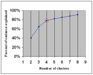
The elbow criterion says that you should choose a number of clusters so that adding another cluster doesn't add sufficient information. More precisely, if you graph the percentage of variance explained by the clusters against the number of clusters, the first clusters will add much information (explain a lot of variance), but at some point the marginal gain will drop, giving an angle in the graph (the elbow).
On the following graph, the elbow is indicated by the red circle. The number of clusters chosen should therefore be 4.
Spectral clustering
Given a set of data points, the similarity matrix may be defined as a matrix where represents a measure of the similarity between point and . Spectral clustering techniques make use of the spectrum of the similarity matrix of the data to cluster the points. Sometimes such techniques are also used to perform dimensionality reduction for clustering in fewer dimensions.


One such technique is the Shi-Malik algorithm, commonly used for image segmentation. It partitions points into two sets based on the eigenvector corresponding to the second-smallest eigenvalue of the Laplacian


of , where is the diagonal matrix


This partitioning may be done in various ways, such as by taking the median of the components in , and placing all points whose component in is greater than in , and the rest in . The algorithm can be used for hierarchical clustering, by repeatedly partitioning the subsets in this fashion.


A related algorithm is the Meila-Shi algorithm, which takes the eigenvectors corresponding to the k largest eigenvalues of the matrix for some k, and then invokes another (e.g. k-means) to cluster points by their respective k components in these eigenvectors.

Applications
Biology
In biology clustering has many applications in the fields of computational biology and bioinformatics, two of which are:
- In transcriptomics, clustering is used to build groups of genes with related expression patterns. Often such groups contain functionally related proteins, such as enzymes for a specific pathway, or genes that are co-regulated. High throughput experiments using expressed sequence tags (ESTs) or DNA microarrays can be a powerful tool for genome annotation, a general aspect of genomics.
- In sequence analysis, clustering is used to group homologous sequences into gene families. This is a very important concept in bioinformatics, and evolutionary biology in general. See evolution by gene duplication.
Marketing research
Cluster analysis is widely used in market research when working with multivariate data from surveys and test panels. Market researchers use cluster analysis to partition the general population of consumers into market segments and to better understand the relationships between different groups of consumers/potential customers.
- Segmenting the market and determining target markets
- Product positioning
- New product development
- Selecting test markets (see : experimental techniques)
Other applications
Social network analysis: In the study of social networks, clustering may be used to recognize communities within large groups of people.
Image segmentation: Clustering can be used to divide a digital image into distinct regions for border detection or object recognition.
Data mining: Many data mining applications involve partitioning data items into related subsets; the marketing applications discussed above represent some examples. Another common application is the division of documents, such as World Wide Web pages, into genres.
Comparisons between data clusterings
There have been several suggestions for a measure of similarity between two clusterings. Such a measure can be used to compare how well different data clustering algorithms perform on a set of data. Many of these measures are derived from the matching matrix (aka confusion matrix), e.g., the Rand measure and the Fowlkes-Mallows Bk measures.
External links
- Jain, Murty and Flynn: Data Clustering: A Review, ACM Comp. Surv., 1999. Available here.
- for another presentation of hierarchical, k-means and fuzzy c-means see this introduction to clustering. Also has an explanation on mixture of Gaussians.
- David Dowe, Mixture Modelling page - other clustering and mixture model links.
- a tutorial on clustering [1]
- The on-line textbook: Information Theory, Inference, and Learning Algorithms, by David J.C. MacKay includes chapters on k-means clustering, soft k-means clustering, and derivations including the E-M algorithm and the variational view of the E-M algorithm.
See also
- k-means
- Artificial neural network (ANN)
- Self-organizing map
- Expectation Maximization (EM)
Bibliography
- Clatworthy, J., Buick, D., Hankins, M., Weinman, J., & Horne, R. (2005). The use and reporting of cluster analysis in health psychology: A review. British Journal of Health Psychology 10: 329-358.
- Romesburg, H. Clarles, Cluster Analysis for Researchers, 2004, 340 pp. ISBN 1411606175 or publisher, reprint of 1990 edition published by Krieger Pub. Co... A Japanese language translation is available from Uchida Rokakuho Publishing Co., Ltd., Tokyo, Japan.
- Heyer, L.J., Kruglyak, S. and Yooseph, S., Exploring Expression Data: Identification and Analysis of Coexpressed Genes, Genome Research 9:1106-1115.
- The on-line textbook: Information Theory, Inference, and Learning Algorithms, by David J.C. MacKay includes chapters on k-means clustering, soft k-means clustering, and derivations including the E-M algorithm and the variational view of the E-M algorithm.
For spectral clustering :
- Jianbo Shi and Jitendra Malik, "Normalized Cuts and Image Segmentation", IEEE Transactions on Pattern Analysis and Machine Intelligence, 22(8), 888-905, August 2000. Available on Jitendra Malik's homepage
- Marina Meila and Jianbo Shi, "Learning Segmentation with Random Walk", Neural Information Processing Systems, NIPS, 2001. Available from Jianbo Shi's homepage
For estimating number of clusters:
- Can, F., Ozkarahan, E. A. (1990) "Concepts and effectiveness of the cover coefficient-based clustering methodology for text databases." ACM Transactions on Database Systems. 15 (4) 483-517.
Software implementations
Free
- the flexclust package for R
- YALE (Yet Another Learning Environment): free open-source software for knowledge discovery and data mining also including a plugin for clustering
- some Matlab source files for clustering here
- COMPACT - Comparative Package for Clustering Assessment (also in Matlab)
- mixmod : Model Based Cluster And Discriminant Analysis. Code in C++, interface with Matlab and Scilab
- LingPipe Clustering Tutorial Tutorial for doing complete- and single-link clustering using LingPipe, a Java text data mining package distributed with source.
- Weka : Weka contains tools for data pre-processing, classification, regression, clustering, association rules, and visualization. It is also well-suited for developing new machine learning schemes.
Non-free
de:Clusteranalyse
hr:Grupiranje
su:Data clustering
th:การแบ่งกลุ่มข้อมูล
| This page uses Creative Commons Licensed content from Wikipedia (view authors). |